Tutorial - Post-process ETABS data

info

Level: Beginners
Time: 20 min

Prerequisites:

• You have an account and completed the installation process. No account? Get one here
• You have some experience with reading Python code

In this tutorial, you will build a VIKTOR app to process and visualize outputs from ETABS. You'll see how to export these outputs from ETABS into a file, upload them into VIKTOR and post-process reaction loads for various load combinations. Along the way, you will work with Plotly and Pandas, using the flexible tools and building blocks that VIKTOR offers.

Here is what we'll cover:

1. Creating an app to take in a file
2. Processing the uploaded .xlsx file exported from ETABS
3. Adding processed data into a field so that the user can select from the results
4. Visualising results based on those selections

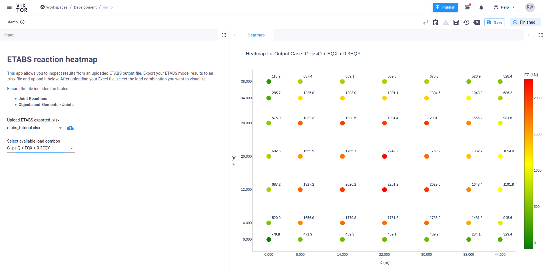
By the end of this tutorial, you will be able to generate a heatmap of the reaction loads for your structure by selecting specific load cases. This will allow you to gain valuable insights from your results and easily share them with your clients and team. Additionally, you will learn how to automate this process using VIKTOR. The final result will look like the figure below:

1. Basic setup

Create an empty app

Let's create, install and start an empty app. This will be the starting point for the rest of the tutorial. But before we start, make sure to shut down any app that is running (like the demo app) by closing the command-line shell (for example Powershell) or end the process using Ctrl + C.

Follow these steps to create, install and start an empty app:

1. Go to the App store in your VIKTOR environment to create a new app. After clicking 'Create app' choose the option 'Create blank app' and enter a name, 'spreadsheet-tutorial', and description of your choice. Submit the form by clicking 'Create and setup'.

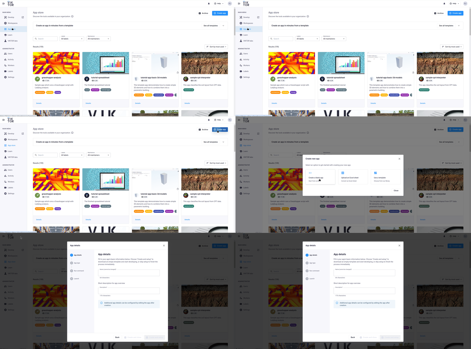
2. Select 'Editor' as app type and click 'Next'.
3. Now follow the instructions to run the quickstart command to download the empty app template. After entering the command click 'I have run the command' to continue. The CLI will ask you to select your code editor of choice. Use the arrows and press enter to select a code editor. The app will now open in your code editor of choice.

If all went well, your empty app is installed and connected to your development workspace. The terminal in your code editor should show something like this:

INFO    : Connecting to cloud.viktor.ai...
INFO    : Connection is established:
INFO    : 
INFO    :     https://cloud.viktor.ai/workspaces/XXX/app  <--- navigate here to find your app
INFO    : 
INFO    : The connection can be closed using Ctrl+C
INFO    : App is ready

Re-starting your app

• You only need create an app template and install it once for each new app you want to make.
• The app will update automatically once you start adding code in app.py, as long as you don't close the terminal or your code editor.
• Did you close your code editor? Use viktor-cli start to start the app again. No need to install, clear, etc.

Adding useful Python packages

We want to use the Python packages Pandas, Openpyxl, and Plotly in this app. Open requirements.txt and add plotly, openpyxl and pandas under your viktor version (don't change that line):

viktor==X.X.X <-- Don't modify this line  
plotly  
pandas
openpyxl

Next, close the connection to your app in the terminal (if the app has been connected automatically). You can do this by using Ctrl+C. Open a new terminal and install the new dependencies (like plotly and pandas) in your Python environment by running this terminal:

viktor-cli install

And after that connect your app to the VIKTOR platform again:

viktor-cli start

Keep the terminal open, as closing it will disconnect your app.

Adding input fields

Let's add some text and input fields for the user to upload their file into. We will include a FileField to upload our .xlsx file and an OptionField to select a load combination from our Excel file.

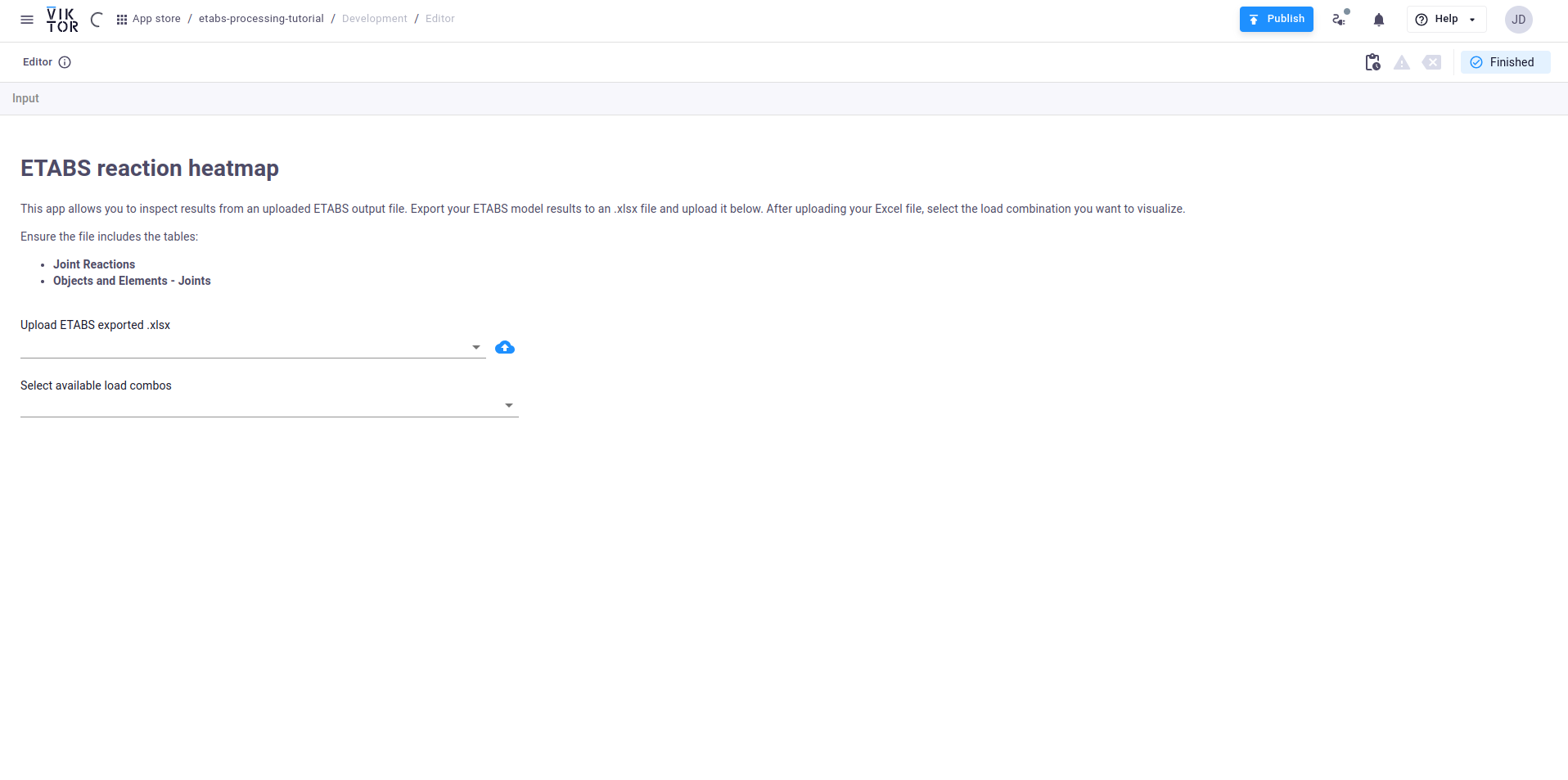
Feel free to copy and paste the highlighted lines code in app.py, save the file and refresh the app in the browser. You should now see the input fields you just added to the code.

import viktor as vkt


class Parametrization(vkt.Parametrization):
    intro = vkt.Text("""
# ETABS reaction heatmap
This app allows you to inspect results from an uploaded ETABS output file. Export your ETABS model results to an .xlsx file and upload it below. After uploading your Excel file, select the load combination you want to visualize.

Ensure the file includes the tables:
- **Joint Reactions**
- **Objects and Elements - Joints**
""")
    xlsx_file = vkt.FileField("Upload ETABS exported .xlsx")
    lb = vkt.LineBreak()
    selected_load_combo = vkt.OptionField("Select available load combos", options=[])


class Controller(vkt.Controller):
    parametrization = Parametrization

The result should look like the image below. Now that the inputs are sorted, we will continue with processing the ETABS data.

2. Process the XLSX file

Sample ETABS exported .xlsx file

For this tutorial, you can use this sample Excel file but don't worry; at the end of this tutorial, we will guide you on how to export this data from ETABS and create your own file.

Processing the uploaded xlsx file

The next step is to process the data from the uploaded Excel file. It's a good idea to do this processing in a separate function, that we'll name process_etabs_file. This function will extract the unique load combinations (which will be used later in our OptionField) and the joint reactions. The goal is to combine this data with the joint coordinates to create a DataFrame that can be used to plot the heatmap in the Plotly view. Below is the logic in the code, along with a breakdown. Add the highlighted lines of code to app.py and save the file.  

import viktor as vkt
import pandas as pd


def process_etabs_file(uploaded_file):
    # Read the file into a dataframe
    sheet_names = ["Joint Reactions", "Objects and Elements - Joints"]
    with uploaded_file.file.open_binary() as fr:
        dataframes = pd.read_excel(fr, sheet_name=sheet_names, skiprows=1)

    # Process the 'Joint Reactions' dataframe
    loads_df = dataframes["Joint Reactions"].dropna(subset=["Unique Name", "Output Case"]).copy()

    # Process the 'Objects and Elements - Joints' dataframe
    cords = dataframes["Objects and Elements - Joints"].dropna(
        subset=["Element Name", "Object Name", "Global X", "Global Y", "Global Z"]
    ).copy()
    cords = cords.rename(columns={"Object Name": "Unique Name"})

    # Get unique load case names as a list
    unique_output_cases = loads_df["Output Case"].unique().tolist()

    # Merge loads and cords dataframe
    merged_df = pd.merge(loads_df, cords, on="Unique Name", how="inner")

    return unique_output_cases, merged_df.reset_index(drop=True)


class Parametrization(vkt.Parametrization):
    intro = vkt.Text("""
# ETABS reaction heatmap
This app allows you to inspect results from an uploaded ETABS output file. Export your ETABS model results to an .xlsx file and upload it below. After uploading your Excel file, select the load combination you want to visualize.

Ensure the file includes the tables:
- **Joint Reactions**
- **Objects and Elements - Joints**
""")
    xlsx_file = vkt.FileField("Upload ETABS exported .xlsx")
    lb = vkt.LineBreak()
    selected_load_combo = vkt.OptionField("Select available load combos", options=[])


class Controller(vkt.Controller):
    parametrization = Parametrization

How this works

1. In the top of the file we import Pandas, which we'll use to load the file content into dataframes
2. The function reads the excel file and extract the necessary sheets: Joint Reactions and Objects and Elements - Joints.
3. Then we filter for and remove the rows that we want based on the required data, keeping columns Global X, Global Y, and Global Z.
4. Finally, merge the processed Joint Reactions data with the joint coordinates using the Unique Name column as the key. This merged DataFrame includes all the necessary information to plot a heatmap.
5. This functions returns two things at once, the unique load combinations and the merged dataframe.

3. Allow user selection of load combinations

With the function to process the uploaded file done, we can now use that processed data in the Parametrization. We will allow users to select a load combination from the unique load combinations. To get the unique load combinations into the OptionField, we can use a callback function. Let's call it get_load_combos. It will get the unique load combinations from read_file and send update our OptionFieldto display a dropdown with the correct options. Add the highlighted lines of code to app.py and don't forget to reference the get_load_combos in the selected_load_combo field.

import viktor as vkt
import pandas as pd


def process_etabs_file(uploaded_file):
    # Read the file into a dataframe
    sheet_names = ["Joint Reactions", "Objects and Elements - Joints"]
    with uploaded_file.file.open_binary() as fr:
        dataframes = pd.read_excel(fr, sheet_name=sheet_names, skiprows=1)

    # Process the 'Joint Reactions' dataframe
    loads_df = dataframes["Joint Reactions"].dropna(subset=["Unique Name", "Output Case"]).copy()

    # Process the 'Objects and Elements - Joints' dataframe
    cords = dataframes["Objects and Elements - Joints"].dropna(
        subset=["Element Name", "Object Name", "Global X", "Global Y", "Global Z"]
    ).copy()
    cords = cords.rename(columns={"Object Name": "Unique Name"})

    # Get unique load case names as a list
    unique_output_cases = loads_df["Output Case"].unique().tolist()

    # Merge loads and cords dataframe
    merged_df = pd.merge(loads_df, cords, on="Unique Name", how="inner")

    return unique_output_cases, merged_df.reset_index(drop=True)


def get_load_combos(params, **kwargs):
    if params.xlsx_file:
        load_combos, _ = process_etabs_file(params.xlsx_file)  # Only use the first returned item, the load_combos
        return load_combos
    return ["First upload a .xlsx file"]


class Parametrization(vkt.Parametrization):
    intro = vkt.Text("""
# ETABS reaction heatmap
This app allows you to inspect results from an uploaded ETABS output file. Export your ETABS model results to an .xlsx file and upload it below. After uploading your Excel file, select the load combination you want to visualize.

Ensure the file includes the tables:
- **Joint Reactions**
- **Objects and Elements - Joints**
""")
    xlsx_file = vkt.FileField("Upload ETABS exported .xlsx")
    lb = vkt.LineBreak()
    selected_load_combo = vkt.OptionField("Select available load combos", options=get_load_combos)


class Controller(vkt.Controller):
    parametrization = Parametrization

By replacing the options=[] with a reference to the callback function (options=get_load_combos) we fill the field with the processed load combos from the file (if there is a file uploaded).

4. Visualize Reaction Loads with Plotly

Once the user selected a load combination, we filter the data to focus on the selected load combination. Then we use Plotly to generate an interactive heat map. To visualize a Plotly figure in a VIKTOR app we can use the add a PloltyView method to the Controller.

We will add a scatter plot to represent each joint from the ETABS Data, with its color indicating the magnitude of the reaction load (FZ). This visualization allows you to clearly observe how loads are distributed across the base floor, making it easier to analyze and interpret the results.

Copy the highlighted piece of code and add it to app.py. Don't forget importing ploty on line 3!

import viktor as vkt
import pandas as pd
import plotly.graph_objects as go


def process_etabs_file(uploaded_file):
    # Read the file into a dataframe
    sheet_names = ["Joint Reactions", "Objects and Elements - Joints"]
    with uploaded_file.file.open_binary() as fr:
        dataframes = pd.read_excel(fr, sheet_name=sheet_names, skiprows=1)

    # Process the 'Joint Reactions' dataframe
    loads_df = dataframes["Joint Reactions"].dropna(subset=["Unique Name", "Output Case"]).copy()

    # Process the 'Objects and Elements - Joints' dataframe
    cords = dataframes["Objects and Elements - Joints"].dropna(
        subset=["Element Name", "Object Name", "Global X", "Global Y", "Global Z"]
    ).copy()
    cords = cords.rename(columns={"Object Name": "Unique Name"})

    # Get unique load case names as a list
    unique_output_cases = loads_df["Output Case"].unique().tolist()

    # Merge loads and cords dataframe
    merged_df = pd.merge(loads_df, cords, on="Unique Name", how="inner")

    return unique_output_cases, merged_df.reset_index(drop=True)


def get_load_combos(params, **kwargs):
    if params.xlsx_file:
        load_combos, _ = process_etabs_file(params.xlsx_file)  # Only use the first returned item, the load_combos
        return load_combos
    return ["First upload a .xlsx file"]


class Parametrization(vkt.Parametrization):
    intro = vkt.Text("""
# ETABS reaction heatmap
This app allows you to inspect results from an uploaded ETABS output file. Export your ETABS model results to an .xlsx file and upload it below. After uploading your Excel file, select the load combination you want to visualize.

Ensure the file includes the tables:
- **Joint Reactions**
- **Objects and Elements - Joints**
""")
    xlsx_file = vkt.FileField("Upload ETABS exported .xlsx")
    lb = vkt.LineBreak()
    selected_load_combo = vkt.OptionField("Select available load combos", options=get_load_combos)


class Controller(vkt.Controller):
    parametrization = Parametrization

    @vkt.PlotlyView("Heatmap")
    def plot_heat_map(params,**kwargs):
        if params.selected_load_combo:
            _, merged_df = process_etabs_file(params.xlsx_file)

            # Filter the dataframe based on the selected load combination
            filtered_df = merged_df[merged_df["Output Case"] == params.selected_load_combo]
            FZ_min, FZ_max = filtered_df["FZ"].min(), filtered_df["FZ"].max()

            # Create plotly scatter plot
            fig = go.Figure(
                data=go.Scatter(
                    x=filtered_df["Global X"],
                    y=filtered_df["Global Y"],
                    mode='markers+text',
                    marker=dict(
                        size=16,
                        color=filtered_df["FZ"],
                        colorscale=[
                            [0, "green"],
                            [0.5, "yellow"],
                            [1, "red"]
                        ],
                        colorbar=dict(title="FZ (kN)"),
                        cmin=FZ_min,
                        cmax=FZ_max
                    ),
                    text=[f"{fz:.1f}" for fz in filtered_df["FZ"]],
                    textposition="top right"
                )
            )

            # Style the plot
            fig.update_layout(
                title=f"Heatmap for Output Case: {params.selected_load_combo}",
                xaxis_title="X (m)",
                yaxis_title="Y (m)",
                plot_bgcolor='rgba(0,0,0,0)',
            )
            fig.update_xaxes(
                linecolor='LightGrey',
                tickvals=filtered_df["Global X"],
                ticktext=[f"{x / 1000:.3f}" for x in filtered_df["Global X"]],
            )
            fig.update_yaxes(
                linecolor='LightGrey',
                tickvals=filtered_df["Global Y"],
                ticktext=[f"{y / 1000:.3f}" for y in filtered_df["Global Y"]],
            )

            return vkt.PlotlyResult(fig.to_json())
        else:
            return vkt.PlotlyResult({})

This code explained

1. At the top of the file, we import Plotly, which we'll use to create the plot
2. At the top of the function, we use process_etabs_file again, only this time we only use the second returned item, the merged dataframe.
3. The dataframe is filtered, based on the selected option in params.load_com. We also find the lowest and highest values for Fz.
4. Using plotly, we create a scatter plot based on the filtere dataframe. Using the lowest and highest values for Fz the colors are determined for each point
5. Finally, we apply some styling to the figure, like adding a title, setting linecolors and text for the tickmarks

The resulting app

Refresh your app in the browser. You will now see the empty graph appear on the right side of the screen. You can now upload the Excel sheet with ETABS loads in the upload field. After that select one of the load combinations, and a heatmap will display the magnitudes, color-coded, along with the joint locations. You can try any combination and test it with any ETABS model. Our final app will look like this:

Complete code

Were you able to do everything in this tutorial without error? If not, you can always look at the full code:

import viktor as vkt
import pandas as pd
import plotly.graph_objects as go


def process_etabs_file(uploaded_file):
    # Read the file into a dataframe
    sheet_names = ["Joint Reactions", "Objects and Elements - Joints"]
    with uploaded_file.file.open_binary() as fr:
        dataframes = pd.read_excel(fr, sheet_name=sheet_names, skiprows=1)

    # Process the 'Joint Reactions' dataframe
    loads_df = dataframes["Joint Reactions"].dropna(subset=["Unique Name", "Output Case"]).copy()

    # Process the 'Objects and Elements - Joints' dataframe
    cords = dataframes["Objects and Elements - Joints"].dropna(
        subset=["Element Name", "Object Name", "Global X", "Global Y", "Global Z"]
    ).copy()
    cords = cords.rename(columns={"Object Name": "Unique Name"})

    # Get unique load case names as a list
    unique_output_cases = loads_df["Output Case"].unique().tolist()

    # Merge loads and cords dataframe
    merged_df = pd.merge(loads_df, cords, on="Unique Name", how="inner")

    return unique_output_cases, merged_df.reset_index(drop=True)


def get_load_combos(params, **kwargs):
    if params.xlsx_file:
        load_combos, _ = process_etabs_file(params.xlsx_file)
        return load_combos
    return ["First upload a .xlsx file"]


class Parametrization(vkt.Parametrization):
    intro = vkt.Text("""
# ETABS reaction heatmap
This app allows you to inspect results from an uploaded ETABS output file. Export your ETABS model results to an .xlsx file and upload it below. After uploading your Excel file, select the load combination you want to visualize.

Ensure the file includes the tables:
- **Joint Reactions**
- **Objects and Elements - Joints**
""")
    xlsx_file = vkt.FileField("Upload ETABS exported .xlsx")
    lb = vkt.LineBreak()
    selected_load_combo = vkt.OptionField("Select available load combos", options=get_load_combos)


class Controller(vkt.Controller):
    parametrization = Parametrization

    @vkt.PlotlyView("Heatmap")
    def plot_heat_map(params,**kwargs):
        if params.selected_load_combo:
            _, merged_df = process_etabs_file(params.xlsx_file)

            # Filter the dataframe based on the selected load combination
            filtered_df = merged_df[merged_df["Output Case"] == params.selected_load_combo]
            FZ_min, FZ_max = filtered_df["FZ"].min(), filtered_df["FZ"].max()

            # Create plotly scatter plot
            fig = go.Figure(
                data=go.Scatter(
                    x=filtered_df["Global X"],
                    y=filtered_df["Global Y"],
                    mode='markers+text',
                    marker=dict(
                        size=16,
                        color=filtered_df["FZ"],
                        colorscale=[
                            [0, "green"],
                            [0.5, "yellow"],
                            [1, "red"]
                        ],
                        colorbar=dict(title="FZ (kN)"),
                        cmin=FZ_min,
                        cmax=FZ_max
                    ),
                    text=[f"{fz:.1f}" for fz in filtered_df["FZ"]],
                    textposition="top right"
                )
            )

            # Style the plot
            fig.update_layout(
                title=f"Heatmap for Output Case: {params.selected_load_combo}",
                xaxis_title="X (m)",
                yaxis_title="Y (m)",
                plot_bgcolor='rgba(0,0,0,0)',
            )
            fig.update_xaxes(
                linecolor='LightGrey',
                tickvals=filtered_df["Global X"],
                ticktext=[f"{x / 1000:.3f}" for x in filtered_df["Global X"]],
            )
            fig.update_yaxes(
                linecolor='LightGrey',
                tickvals=filtered_df["Global Y"],
                ticktext=[f"{y / 1000:.3f}" for y in filtered_df["Global Y"]],
            )

            return vkt.PlotlyResult(fig.to_json())
        else:
            return vkt.PlotlyResult({})

Export your own results from ETABS

If you want to try this app with your own data, first run your analysis and then export the reaction loads from your ETABS model. Navigate to File menu > Export > ETABS Tables to Excel within ETABS, and select the Joint Reactions and Objects and Elements - Joints tables, as shown in the figure below:

warning

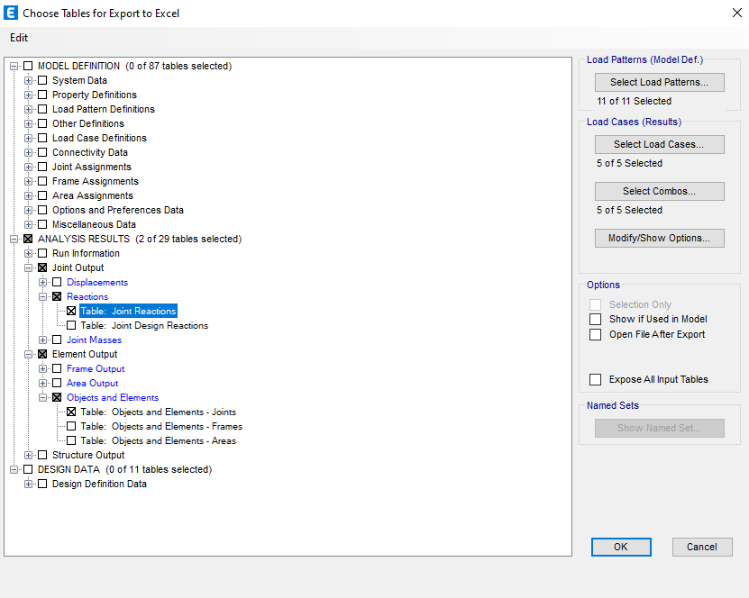
Ensure that your exported Excel file contains these specific sheets. Without them, the app won’t be able to read and process the data correctly. Set the model units to international system units. The model expects the loads in kN and in millimeters (mm).

What's next?

In this tutorial, you learned how to post-process results exported from ETABS. Your next goal could be to implement automation using the CSI API from your VIKTOR app. To achieve this, the best place to start is the following tutorial.

If you want to explore more use cases where VIKTOR shines, feel free to check out our other tutorials!